Probability Distributions
In this section we’re going to learn about some common probability distributions
Watch the video and then answer the questions below.
Thirteen-minute video
You can also view this video on YouTube
You can find the slides here and also as .odp.
Key Points
Discrete Random Variables
A variable that has a countable number of possible values is called a discrete random variable If you roll a dice, there are a countable number of possible values:
⚀ ⚁ ⚂ ⚃ ⚄ ⚅
The list of probabilities for each value is the probability function or probability mass function. This gives its probability distribution. The list of probabilities must add up to 1.
Discrete probability distributions include:
- Binomial distribution
- Poisson distribution
Continuous Random Variables
A variable that could take an infinite (continuous) number of values is a continuous random variable. For example, the height of a random student might be a continuous random varible.
It is represented by the area under a curve, or integral. This curve is a probability density function. The area under the curve adds up to 1. There are an infinite number of possible values, so the probability of any single value is 0.
Continuous probability distributions include:
- Normal distribution
- Exponential distribution
Uniform Distribution
All outcomes are equally likely. Like rolling a fair dice.

In the case of a discrete uniform distribution, if there are \( n \) outcomes, the probability for each outcome is:
\[ P(X=x)= \frac{1}{n} \]
In the case of a uniformly distributed variable that takes values between \( a \) and \( b \), its probability density function is:
\[ f(x) = \begin{cases} \frac{1}{b-a} & a \leq x \leq b \\ 0 & x \lt b \textrm{ or } x \gt b \end{cases} \]
Binomial Distribution
Models the number of successes for boolean data: coin flips, yes/no questions, etc.
Its probability mass function is the following:
\[ P(X=x)=^nC_x \times p^x \times (1-p)^{(n-x)} \]
Normal Distribution
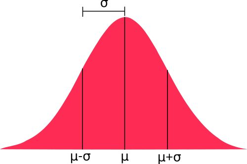
Also known as the Gaussian distribution. The classic bell curve. Very common in real-world data.

It is defined by its mean \( \mu \) and standard deviation \( \sigma \). These are the only two parameters you need to know to plot a normal distribution. As it is defined by parameters, it is a parametric distribution.
It’s probability density function is the following:
\[ f(x)=\frac{1}{\sigma\sqrt{2\pi}}e^{-\frac{1}{2}(\frac{x - \mu}{\sigma})^2} \]
Which looks complicated, but remember it’s just a function of \( \mu \) and \( \sigma \).
Remember, because it’s continuous, if you wanted to find the probability of a range of values, you’d have to use integration to find the area under the curve.
Questions
1. Check your understanding
| Expression | Discrete | Continuous | ||
|---|---|---|---|---|
| 1. | Rolling a biased dice | |||
| 2. | Java’s Math.random() |
|||
| 3. | A random integer 0-100 |
|||
| 4. | A binomial distribution | |||
| 5. | A normal distribution |
Summary
In this section we have learned about probability distibutions.
In the next section we get on to samples and populations.